A journey from scratch to Diffusion. Principles and directions.

Introduction to the concepts underlying diffusion and comparison of the main techniques.

Updates

• [16/02/2023] Added my notes on Universal Guidance for Diffusion Models!

Introduction

Source: (Vahdat et al. 2022)

In Deep Learning, generative models learn and sample from a (usually) multivariate distribution. Auto-encoders (AE) are part of a class of algorithms usually designed with smaller hidden layers, an “information bottleneck”, which force learning “compressed” representations of data. With this approach, the learned distribution results sparse and possibly overfitted: Variational Auto Encoders (VAE) tackle this issue as they force to model latent representations with a probability distribution, such as a multi-variate Gaussian, for more smoothness.

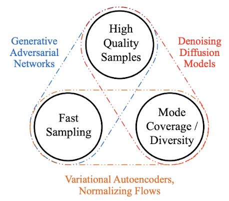
Diffusion (Sohl-Dickstein et al., 2015) is inspired by thermodynamics and over the last 2-3 years it has become a very popular approach. Compared to Generative Adversarial Networks (GANs), VAE and AE, Diffusion allows a tradeoff between speed of sampling, fidelity and coverage of the data distribution (figure 1), the approach consists in noising/denoising processes of usually-high dimensional feature vectors.

This post aims to provide a broad and complete overview from the foundations to the most crucial achievements. I will not dive in derivations and mathematical intuition, which are covered in this excellent post by Lilian Weng. To explore further learning resources and applications, I suggest this rich github repo and this survey.

Learning a data distribution: Metropolis-Hastings Markov Chains

From literature, the building blocks for Diffusion consists in topics from statistics, stochastic optimization and machine learning. While we don’t know the density of a target data distribution the Metropolis-Hastings algorithm (MH) comes to help to generate samples approximating that distribution. Such samples are generated according to a Markov Chain.

A Markov chain (MC) is a sequence of random variables $x_{t}$, where $x_{t} \rightarrow x_{t+1}$ according to a defined transition function. With MH, we can use MC to approximate the data distribution $p(x)$ by generating randomly (Markov-chain Monte-Carlo) some “acceptable” samples.

This algorithm designs a Markov chain such that its stationary distribution $\pi(x)$ is $p(x)$ by assuming that $\pi(x)$ exists and it is unique.

1. Initialize $x_{t=0}$ , define a proposal approximating distribution $g(x) \approx p(x)$
2. Generate a candidate $x^* $ from $Q(x^* \mid x_{t}$). For a random walk transition: $x^* = x_t + \mathcal{N}(0, \sigma^2 I)$ , in this case $Q(x)$ is symmetric → $Q(x^* \mid x_t)=Q(x_t\mid x^* )$.
3. Compute the acceptance probability $A=\min (1, \frac{g(x^* ) Q(x_t \mid x^* )}{g(x_t) Q(x^* \mid x_t)})$, when $Q(x)$ is symmetric it reduces to: $A=\min (1, \frac{g(x^* ) }{g(x_t) })$. With probability $A$, accept $x_{t+1} = x^* $ (intuitively such that $g(x^* )$ shall be large enough compared to $g(x_t)$), otherwise $x_{t+1} = x_t$.
4. Repeat 2-3 to produce samples.

Learning a data distribution: Stochastic Gradient Langevin Dynamics

(Welling et al., 2011) propose an iterative method to learn a distribution $p(x)$ with small batches of training data samples: Stochastic Gradient Langevin Dynamics (SGLD).

• Stochastic Differential Equations (SDE) can be used for density estimation (Milstein et al. 2004), as their equilibrium distribution approximates a target $p(x)$. Langevin equations belong to the family of SDEs, and their application to Monte-Carlo simulations, Langevin dynamics, propose a discretization and approximation method.

• In stochastic optimization, the parameters $\theta^* $ of a model $p(x \mid \theta)$ can be estimated with Maximum A Posteriori (MAP), $p(\theta\mid X) \propto p(\theta) \prod_{i=1}^N p(x_i \mid \theta)$ . With stochastic gradient descent, the parameter update equals :

  \[\begin{aligned} \Delta \theta_t &=\frac{\epsilon_t}{2}(\nabla \log p(\theta_t)+\sum_{i=1}^N \nabla \log p(x_i \mid \theta_t))+\eta_t, \eta_t \sim N(0, \epsilon) \end{aligned}\]

  As illustrated, the update is actually computed using a subset of the training set $X_t = {x_{t1},… , x_{tn}}$ iteratively for steps $t$ ,with $\epsilon_{t} \rightarrow0$ step size . In order to avoid collapsing to local minima, we account for uncertainty by injecting gaussian noise $\eta_t \sim N(0, \epsilon)$ (we are using “random walks” as in Metropolis Hastings to explore the parameters space).

For $t \rightarrow+\infty$, $\epsilon_t \rightarrow0$, this expression converges to Langevin dynamics. Moreover, stochastic gradient noise will average out (gradients for a subset will converge to the gradients of the complete training set) and the discretization error in Langevin dynamics will converge to zero (also the Metropolis Hastings rejection rate converges to zero).

Generative behavior with score matching and noise-conditional score-networks (NCSN)

The sampling process above shown thus leverages Langevin Dynamics. Given a data distribution $p(x)$ , samples are generated with random walks guided with the score function $\nabla_{\mathbf{x}}\log p(x_{t-1})$:

\[\mathbf{x}_t=\mathbf{x}_{t-1}+\frac{\epsilon_t}{2} \nabla_{\mathbf{x}} \log p(\mathbf{x}_{t-1})+\sqrt{\epsilon_t} \boldsymbol{\eta}_t, \quad \text { where } \boldsymbol{\eta}_t \sim \mathcal{N}(\mathbf{0}, \mathbf{I})\]

(Song, Ermon, 2019) suggest the use of a neural network as approximation $s_{\theta}(x)\approx \nabla_{\mathbf{x}}\log p(x)$ (score matching), such approach takes the name of score-based generative modeling. The objective consists in minimizing the cost function in two possible (equivalent) forms:

\[\frac{1}{2} \mathbb{E}_{p_{\text {data }}}[\mathbf{s}_{\boldsymbol{\theta}}(\mathbf{x})-\nabla_{\mathbf{x}} \log p_{\text {data }}(\mathbf{x})_2^2] = \mathbb{E}_{p_{\text {data }}(\mathbf{x})}[\operatorname{tr}(\nabla_{\mathbf{x}} \mathbf{s}_{\boldsymbol{\theta}}(\mathbf{x}))+\frac{1}{2}\mathbf{s}_{\boldsymbol{\theta}}(\mathbf{x})_2^2]\]

However, computing $\operatorname{tr}(\nabla_{\mathbf{x}} \mathbf{s}_{\boldsymbol{\theta}}(\mathbf{x}))$ can be expensive with high dimensional data (large gradient vector), two possibilities follow:

• Denoising score matching: add noise to a data point $x$ and compute the score on the perturbed distribution $q_\sigma(\tilde{\mathbf{x}} \mid \mathbf{x})$, instead of the approximated score function $s_{\theta}(x)$.
• Sliced score matching: the costly trace function is approximated with a series of vector projections, $tr(\nabla_x) s_{\theta}(x))\approx v^{T} \nabla_{x} s_{\theta}(x) v$. The score is computed on the unperturbed data distribution, but it costs 4x the computation since projections require forward mode auto-differentiation.

One challenge for score-based generative modeling is dictated by the manifold hypothesis: high-dimensional features in the real data distribution can be learned in a low-dimensional latent spaces (a manifold). However, the score function is not defined for that manifold, plus the score matching function is a consistent estimator of the distribution for the high-dimensional space.

(Song, Ermon, 2020) propose an improved sampling technique leveraging Annealed Langevin Dynamics, briefly: the data is perturbed with Gaussian noise in order to prevent the resulting distribution to collapse to a low-dimensional manifold; samples in low-density region are produced.

This approach results in Noise Conditional Score Networks: with series of noise variances (std. dev.) $\sigma_i_{i=0}^L$ that satisfies the property $\frac{\sigma_1}{\sigma_2} = … = \frac{\sigma_{L-1}}{\sigma_L} > 1$, a network $s_\theta(x_t, \sigma)$ is trained to predict the score at various noise scales.

Probabilistic Diffusion Models

Deep Denoising Probabilistic Models (DDPM)

Diffusion Models in the modern, most referred variant are probabilistic models (Ho et al. 2020). This architecture takes as input data tensors a gives in output tensors of the same length. The model learns the distribution of the training by noising each sample/batch and predicting how to denoise it:

• Forward process: gradual gaussian noise is added to a sample $x_0$ for $x_{1:T}$ (forward process). With an increasingly large variance $\beta_{t}$, $x_t$ should eventually have an isotropic gaussian distribution (diagonal covariance matrix).

\[q(\mathbf{x}_{1: T} \mid \mathbf{x}_0):=\prod_{t=1}^T q(\mathbf{x}_t \mid \mathbf{x}_{t-1}), \quad q(\mathbf{x}_t \mid \mathbf{x}_{t-1}):=\mathcal{N}(\mathbf{x}_t ; \sqrt{1-\beta_t} \mathbf{x}_{t-1}, \beta_t \mathbf{I})\]

With $\beta_{0:T}$ a variance schedule. A noisy sample $x_t$ can be directly computed with $\alpha_t = 1 - \beta_t$, $\bar{\alpha_t} := \prod_{s=1}^{t} \alpha_s$ :

\[\quad q(\mathbf{x}_t \mid \mathbf{x}_{0}):=\mathcal{N}(\mathbf{x}_t ; \sqrt{\bar{\alpha}_t} \mathbf{x}_{t-1}, (1-\bar{\alpha}_t) \mathbf{I})\]

• Reverse process: with $x_t$, the network predicts the noise to subtract in order to compute the unperturbed, approximately original $\tilde{x_0}$ iteratively:

  \[p_\theta\left(\mathbf{x}_{0: T}\right):=p\left(\mathbf{x}_T\right) \prod_{t=1}^T p_\theta\left(\mathbf{x}_{t-1} \mid \mathbf{x}_t\right), \quad p_\theta\left(\mathbf{x}_{t-1} \mid \mathbf{x}_t\right):=\mathcal{N}\left(\mathbf{x}_{t-1} ; \boldsymbol{\mu}_\theta\left(\mathbf{x}_t, t\right), \mathbf{\Sigma}_\theta\left(\mathbf{x}_t, t\right)\right)\]

  $x_{t-1}$ is sampled from a gaussian with estimated (by the neural network) $\mu_\theta$ and $\Sigma_\theta$ parameters. However, (Ho et al., 2020) actually suggest to predict the added noise with a predictor $\epsilon_\theta$, from which you can derive $\mu_\theta$ , $\Sigma_\theta$ is scheduled. A simplified optimization objective is proposed, as claimed to be more effective than other approaches (eg. loss based on a variational lower bound):

  \[L_{simple} := E_{t \sim[1,T], x_{0} \sim q(x_{0}), \epsilon \sim N(0,I)}[\vert\vert\epsilon-\epsilon_\theta(x_{t},t)\vert\vert^{2}]\]

This is shown to be equivalent to denoising score-matching, where the score function is approximated with the noise predictor: $\nabla_{\mathbf{x}}\log p(x_{t}) \propto \epsilon_\theta(x_t, t)$.

For generative behavior, random gaussian noise is sampled $u_t$ with the same dimensionality of $x_t$, or either $x_t$is used, and the sampling process is applied. It is possible to influence such de-noising process with other information (conditioning), i.e.: text prompts, images, descriptive features.

Improved DDPM

To enhance the sampling capacities, the above mentioned methods can be generalized with Stochastic Differential Equations (SDE), as proposed in (Song et.al, 2021): instead of perturbing the input signal in finite, discrete steps, data points are diffused into noise with a continuum of evolving distributions. Perturbed and denoised samples are thus computed with numerical SDE solvers:

• The SDE for the forward process $x_{0:T}$ is defined as:

\[{\frac{\partial x}{\partial t}}=f(x,t)+\sigma(t)\omega_{t}\Longleftrightarrow\partial x=f(x,t)\cdot\partial t+\sigma(t)\cdot\partial\omega\]

Where $\omega_t$ is Gaussian noise, $f$ is the drift coefficient and $\sigma$ is the diffusion coefficient.

• The reverse-time SDE for the reverse process $x_{t:0}$ is defined as:

\[\partial x=[f(x,t)-\sigma(t)^{2}\cdot\nabla_{x}\log p_{t}(x)]\partial t+\sigma(t)\partial\hat{\omega}\]

With Brownian motion $\hat{\omega}$. Note that $\nabla_{\mathbf{x}}\log p_t(x)$ is the score function of the density at a given time step, by score matching a neural network is applied: $s_{\theta}(x)\approx \nabla_{\mathbf{x}}\log p_t(x)$. A continuous version of the optimization objective is adopted:

\[L_{dsm}^* = R_{t} [\lambda(t) \vert E_{p(x(0))} \vert E_{p_{t}(x(t) \vert x(0))} \vert\vert S_{\theta}(x,t) - \nabla_{x} \log p_{t}(x_{t} \vert x_{0})\vert\vert _{2}^{2}]\]

With $\lambda(t), t \sim U(0, T)$ a weighting function wrt. time.

As further improvement, the paper (Song et.al, 2021) also introduces the Predictor-Corrector (PC) sampler to correct the sampling process with a score-based method such as Annealed Langevin Dynamics. Ordinary Differential Equations (ODE) are also applied to formulate novel and more efficient samplers.

A small note on metrics

There are two measures that will be used in the following research literature to evaluate generative models:

• IS (Inception Score): a measure for class variety and sample unicity in the generated samples.
• FID (Fréchet Inception Distance): Frechét distance between the generated and the original samples. Both fed to an Inception v3 network (similarly to how human neurons process abstract concepts), the metric is computed on the mean and std. dev. of the logits of the deepest layer.

Deterministic Diffusion Models

Deep Denoising Implicit Models (DDIM)

To generate samples, DDPMs involve an iterative, possibly costly sampling procedure which relies on Markov Chains.

Source: [Song et al., 2020]

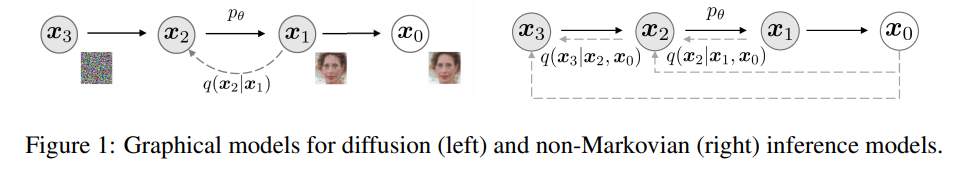
(Song et al., 2020) generalize noising and sampling with non-Markovian processes and seek to achieve a tradeoff between stochasticity and sampling length for speed.

• Forward process: multiple inference distributions indexed by the std. dev. vector $\sigma \in \mathbb{R}_{\ge 0}^T$

  \[q_{\sigma}(x_{1;T}|x_{0}):=q_{\sigma}(x_{T}|x_{0})\prod_{t=2}^{T}q_{\sigma}(x_{t-1}|x_{t},x_{0})\]

  Where $q(x_T \mid x_0):=N(\sqrt{\alpha_T}x_0, (1-\alpha_{t}) I)$ and for all $t>1$,

  \[q_{\sigma}(x_{t-1} \vert x_{t}, x_{0}) = N (\sqrt{\alpha_{t-1}} x_{0} + \sqrt{1-\alpha_{t-1}-\sigma_{t}^{2}} \cdot {\frac{x_{t}-\sqrt{\alpha_{t}}} x_{0}} {\sqrt{1-\alpha_{t}}}, \sigma_{t}^{2}{1})\]

  The forward process derives from the Bayes’ rule:

  \[q_{\sigma}(x_{t}|x_{t-1},x_{0})=\frac{q_{\sigma}(x_{t-1}|x_{t},x_{0})q_{\sigma}(x_{t}|x_{0})}{q_{\sigma}(x_{t-1}|x_{0})}\]

  Such process is no longer Markovian, since $x_t$ could depend on both $x_{t-1}, x_0$. The magnitude of $\sigma$ determines the stochasticity of the forward process.

• Reverse process: the sampling distribution $p_\theta^{(t)}(x_{t-1}\mid x_t)$ leverages knowledge from $q_\sigma(x_{t-1} \mid x}t, x_0)$; in order to sample $x{t-1}$, $x_t$ and a prediction of $x_0$ are required:

  \[f_{\theta}^{(t)}(x_{t}):=(x_{t}-\sqrt{1-\alpha_{t}}\cdot\epsilon_{\theta}^{(t)}(\alpha_{t}))/\sqrt{\alpha_{l}}\] \[p_{\theta} ^ {(t)} (x_{t-1}|x_{t}) = \begin{array}{l l} {N(f_{\theta}^{(1)}(x_{1}),\sigma_{1}^{2}I)} & {\mathrm{if} t=1} \\ {q_{\sigma}(x_{t-1}|x_{t},f_{\theta}^{(t)}(x_{t}))} & {\mathrm{otherwise}} \end{array}\]

  Where $q_\sigma(x_{t-1} \mid x_t, f_\theta^{(t)}(x_t))$ is the equation above with $x_0$ replaced.

For the optimization objective, $\sigma \in \mathbb{R}^T_{\ge0}$ suggests multiple models to be trained with different variances.

\(J_{\sigma}(\epsilon_{\theta}):= E_{x_{0}:T\sim q_{\sigma}(x_{0},z)}[\log q_{\sigma}(x_{1:T}|x_{0})-\log p_{\theta}(x_{0:T})]\) \(= E_{x_{0},\,r\sim q_{\sigma}\,(x_{0},\,r)}\left[\log q_{\sigma}(x_{T}|x_{0})+\sum_{t=2}^{T}\log q_{\sigma}(x_{t-1}|x_{t},x_{0})-\sum_{t=1}^{T}\log p_{\sigma}^{(t)}(x_{t-1}|x_{t})-\log p_{\theta}(x_{T})\right]\)

However, the paper introduces a theorem:

\[{\mathrm{Theorem~I.}}~F o r\,a l l\,\sigma\gt 0,\,t h e r e~e x i s t s\gamma\in\mathbb{R}_{\mathrm{\tiny{r}o l}}^{r}\,a n d\,C\in\mathbb{R}_{\mathrm{\tiny{r}o}}^{r}\,a n d\,C\in\mathbb{R}_{\mathrm{\tiny{r}o}}\,s u c h\,t h a t\,J_{\sigma}=L_{\gamma}+C.\]

Meaning when the weights of the network $\epsilon_\theta^{(t)}$ are not shared across different $t$ steps, $L_1$ from DDPMs is used as a surrogate objective for variational inference $J_\sigma$.

Therefore, the paper suggests involving pre-trained probabilistic diffusion models (DDPM) in non-Markovian processes to noise and denoise data points.

From $p_\theta(x_{1:T})$, a sample $x_{t-1}$ can be generated from $x_t$ via:

\[x_{t-1}={\sqrt{\alpha_{t-1}}}\left({\frac{x_{t}-{\sqrt{1-\alpha_{t}}}\epsilon_{\theta}^{(t)}(x_{t})}{\sqrt{\alpha_{t}}}}\right)+{\sqrt{1-\alpha_{t-1}-\sigma_{t}^{2}}}\cdot\epsilon_{\theta}^{(t)}(x_{t})+\underbrace{\sigma_{t}\epsilon_{t}}_{\mathrm{randon}}\left(\frac{x_{t}}{x_{t}}{x_{t}}\right)\left(1-\alpha_{t}-\beta_{t}^{\alpha_{t}}\right)\]

As previously mentioned, notice when $\sigma_t \rightarrow 0$, sampling becomes deterministic. In the experiments, the authors of (Song et al., 2020) “modulate” stochasticity with $\eta$ defined in:

\[\sigma_{\tau_{i}}(\eta)=\eta\sqrt{(1-\alpha_{\tau_{i-1}})/(1-\alpha_{\tau_{i}})}\sqrt{1-\alpha_{\tau_{i}}/\alpha_{\tau_{i-1}}}\]

Where ${x_{\tau_1},…, x_{\tau_S}}$ is a subset of latent variables and its reverse process is the sampling trajectory. Noising and de-noising a smaller sequence of variables is possible due to the properties of $L_1$ , thus sampling is significantly improved on subsequences of length $S<T$ .

Performance compared with DDPM

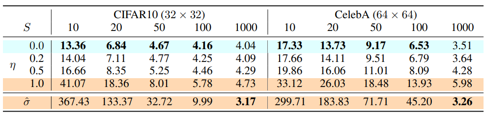
1. With $\eta$ as hyperparameter for stochasticity, $S$ for sequence length, experiments in (Song et al., 2020) emphasize the sampling efficiency of DDIM (deterministic, $\eta = 0$), which matches the quality of DDPM ($\eta > 0$) in 1000 steps with 10x, 20x smaller sequences.
2. Moreover, DDIM are shown to satisfy a consistency property: for the same latent variable $x_t$, multiple samples produced have similar high level features, denoting interpolation capabilities.

Generalized diffusion models (hot, cold diffusion)

(Bansal et al., 2022) throws into discussion the current understanding on diffusion models by testing deterministic transformations with supporting results. The claim is that generalized behavior does not depend on the denoising operator, some proof is provided below.

Their major contributions consist in an improved sampling algorithm and a generalized framework to expand diffusion to deterministic transformations and improve density estimation.

note: the above mentioned forward and reverse processes are renamed as degradation $D(x_0,t)$ and restoration $R_\theta(x_t,t)$, function-wise.

The simple objective becomes:

\[min_\theta \mathbb{E}_{x \sim X} \mid \mid R_\theta(D(x,t),t)-x\mid \mid\]

Where $x \in \mathbb{R}^n$ is an image firstly subject to degradation and then restoration.

For improved generation, probabilistic diffusion models denoise the latent variable $x_t$ and add noise back at each step (but it decreases over time). One could tell the restoration operation actually consists in:

• An estimation $R(x_t,t) = \hat{x_0}$
• Effective denoising through $D(\hat{x_0}, t-1) = x_{t-1}$

Summarized in the algorithm below:

Source: [Song et al., 2020]

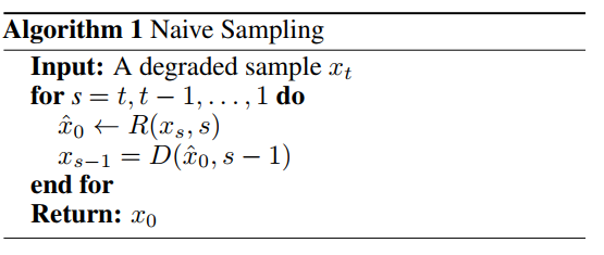
Recalling DDPM, we rewrite line 2 with:

\[\hat{x_0} \rightarrow (x_s-\epsilon_{\theta}(x_s,s))=R(x_s,s)\]

The estimation (restoration) of $x_0$ is perfect because the network $\epsilon_{\theta}(x_s,s)$ is trained to correct for errors and to move towards $x_{s-1}$, but what happens with deterministic, imperfect restorations? → $\hat{x_0}$ accumulates errors → $x_{s-1}$ diverges from the distribution.

An improved sampling algorithm is proposed:

Source: [Song et al., 2020]

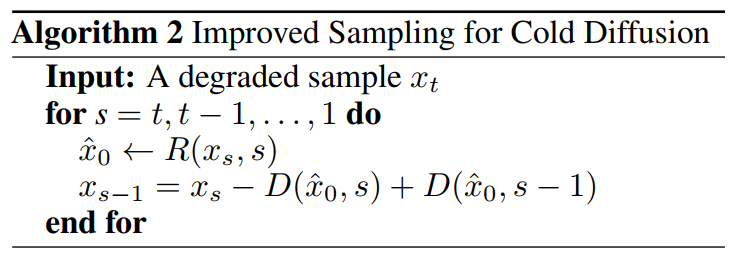
It accounts and tolerates errors in restoration $R$. As proof, consider a linear degradation function $D(x,s) \approx x + s \cdot e$. The process in line 3 is rewritten as:

\[\begin{array}{l}{x_{s-1}=x_{s}-D(R(x_{s},s),s)+D(R(x_{s},s),s-1)}\\ {=D(x_{0},s)-D(R(x_{s},s),s)+D(R(x_{s},s),s-1)}\\ {=x_{0}+(s-1)\cdot e}\\ {=D(x_{0},s-1)}\end{array}\]

This means the choice of $R$ is irrelevant, the restoration would occur the same way as $R$ were perfect or not. Several degradations are tested:

• Blurring
• Pixel masking
• 2x downsampling
• Snowification

For generative behavior, DDPM benefit from the fact that the noisy, latent variable $x_t$ is an isotropic Gaussian, thus it is possible to sample a random point and apply the denoising iteration.

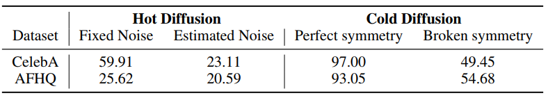
For deterministic transformations, the latent variable $x_t$ is modeled with an appropriate distribution to similarly sample a random point and perform restoration. In case of blurring, $x_t$ is found to be constant (same color for every pixel) for large $T$, since such color is the mean of the RGB image $x_0$, you can use a gaussian mixture model (GMM) to sample random $\hat{x_t}$. Such technique yields high fidelity but low diversity (perfect symmetry) to the training data distribution, thus a small amount of Gaussian noise is added to each sampled $\hat{x_t}$, with drastically better results.

Results show cold diffusion (deterministic, where hot = highest stochasticity) achieves higher Fréchet Inception Distance (FID) (lower distance from the training set in variety and details), suggesting better learning capabilities.

Source: [Song et al., 2020]

As Philip Weng (lucidrains) states on the unofficial DDPM repo: “(…) Turns out none of the technicalities really matters at all”. This approach opens new ways for better generation and density estimation capabilities for diffusion models.

Latent “Stable” Diffusion

Diffusion models originally process high-dimensional data throughout the pipeline, thus it is easy to deduct this approach becomes computationally expensive with small images (i.e. 500x500). (Rombach et al., 2022) disentangles learning of high-level features in likelihood-based models in two stages: perceptual compression, the model cuts out high frequencies (usually useless details); semantic compression, the model actually learns semantic and conceptual composition of data features.

With proper objective function design, Diffusion Models can avoid learning high frequency meaningless information, however all the image pixels are still processed.

Source: Rombach et al., 2022

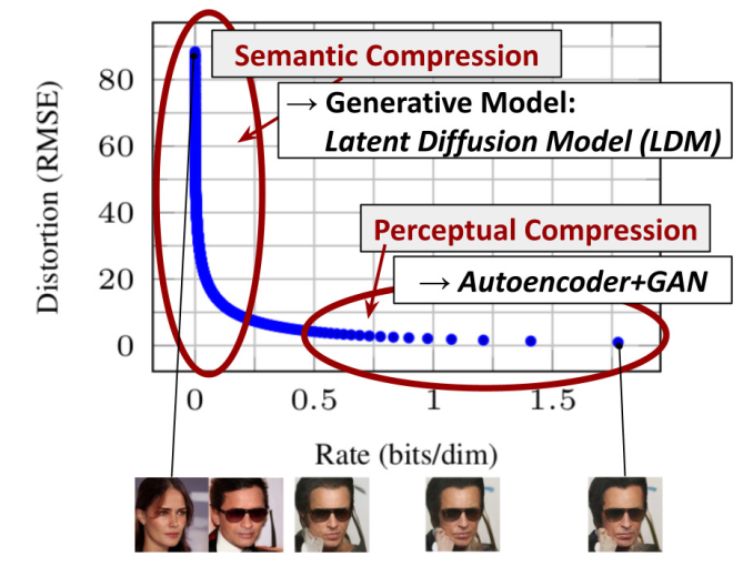
Consequently, (Rombach et al., 2022) introduce Latent Diffusion Models, featuring a two-step framework:

• An autoencoder to compress/de-compress high-dimensional data with controllable compression factors ($\mathcal{E}(x)$ the encoder, mainly a VQ-GAN from (Esser et al., 2021), $\mathcal{D}(x)$ the decoder).
• A diffusion model applied on latent vectors generated by the encoder $\mathcal{E}(x)$. The “layers” in this DM consist in a UNet architecture (Ronneberger et al., 2015) with cross-attention, which allows conditioning with a vector of any modality (text, images, masks) from a backbone $\tau_\theta(y)$ (i.e. a language model with a prompt $y$).

The objective derived from DDPM involves a noise predictor network $\epsilon_\theta(z_t, t, \tau_\theta(y))$ :

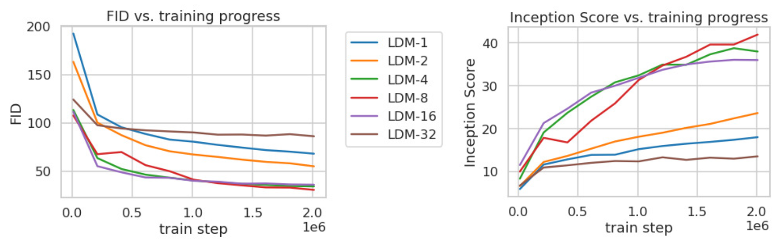
\[{\cal L}_{L D M} := \mathbb{E}\varepsilon(x),y,\epsilon\sim N(0,1),t[||\epsilon-\epsilon_\theta(z_{t},t,\tau_{\theta}(y))||^{2}]\]

With this approach, degradation and (restoration) sampling in Diffusion Models are drastically improved as the computed vectors are much smaller. Experiments in (Rombach et al., 2022) show variable FID scores wrt. the training steps and the downsampling (compression) factor $f = {2,…,32}$ of the autoencoder $(\mathcal{E}(x), \mathcal{D}(x))$.

We also report the image synthesis compared performance:

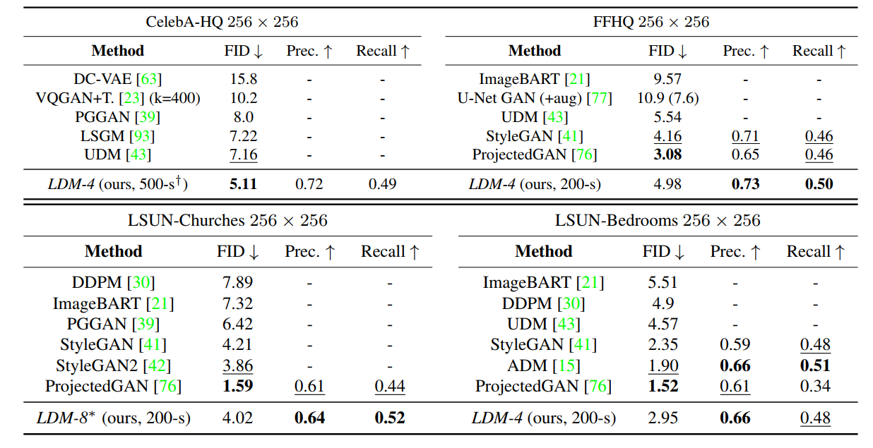
For further details: High-Resolution Image Synthesis with Latent Diffusion Models.

Possibly, a next step could be including this approach to Generalized Diffusion Models and test the (conditioned) generation behavior of deterministic diffusion models.

Conditioned, Guided sampling in Diffusion Models

To generate new samples from the learned distribution $\hat{p}(x)$, we apply the diffusion reverse (denoising) process to a random point $x_t$. It is possible to guide this process with additional information such as captions, images, segmentation masks etc.

• With conditioning, e.g. image/text tokens are provided as additional input to the denoising network $\epsilon_{\theta}$, which usually needs to be trained.
• With guidance, sampling is oriented with the gradients of some “scoring function” such as text-image matching with CLIP.

Classifier guidance

(Dhariwal, Nichol, 2021) propose to guide sampling in diffusion models with noise labels from a trained classifier $p_\phi(y \mid x_t)$ (eg. a ResNet classifying noisy samples as dog images). In DDPM, the next slightly denoised vector is sampled from the distribution:

\[p_\theta(x_t \mid x_{t-1}) = \mathcal{N}(\mu,\Sigma) \\ p_{\theta,\phi}(x_t \mid x_{t+1},y) = Zp_\theta(x_t \mid x_{t+1})p_\phi(y \mid x_t)\]

Where $\mu, \Sigma$ are predicted with a neural network, $Z$ is a normalizing constant. However, sampling from the above distribution is usually intractable, (Sohl-Dickstein et al., 2015) suggest using a perturbed Gaussian distribution; classifier-guidance is summarized with the algorithm:

Source: Dhariwal, Nichol, 2021.

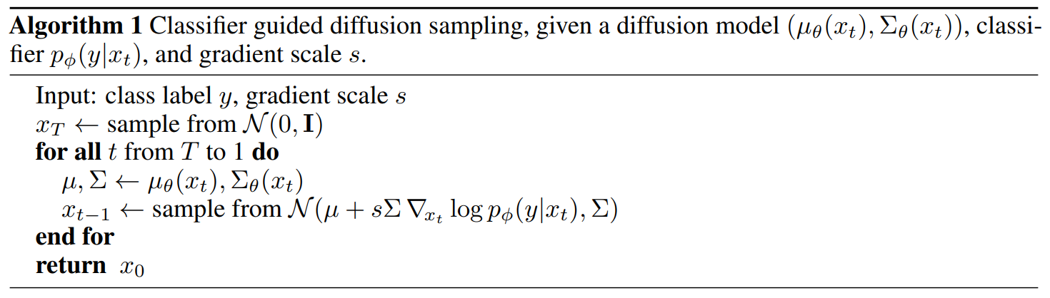
In a very simplified way, I see it as: “the classifier guides sampling from the learned distribution with directions (the gradient) pointing towards the area of the space that make sense to the classifier itself”.

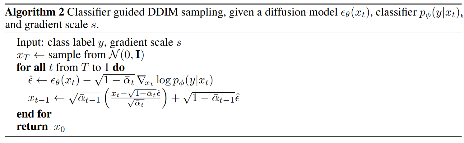
Throwing away random walks in DDIM, a different algorithm is adopted: as mentioned above, score-matching and diffusion models are linked (Song, Ermon, 2019), thus we can derive the conditioned noise predictor with the score-matching trick (Song et al. 2020). The score function is expressed in terms of the noise predictor:

\[\begin{aligned}\nabla_{x_{t}} \log (p_{\theta}(x_{t}) ) &=-\frac{1}{\sqrt{1-\bar{\alpha}_{t}}} \epsilon_{\theta}(x_{t})\end{aligned}\]

For classifier guidance, we consider the score of the joint probability:

\[\begin{aligned}\nabla_{x_{t}} \log (p_{\theta}(x_{t}) p_{\phi}(y \mid x_{t})) &=\nabla_{x_{t}} \log p_{\theta}(x_{t})+\nabla_{x_{t}} \log p_{\phi}(y \mid x_{t}) \\&=-\frac{1}{\sqrt{1-\bar{\alpha}_{t}}} \epsilon_{\theta}(x_{t})+\nabla_{x_{t}} \log p_{\phi}(y \mid x_{t})\end{aligned}\]

Finally, the score of the joint distribution is seen as the classifier-guided noise predictor:

\[\hat{\epsilon}(x_{t}):=\epsilon_{\theta}(x_{t})-\sqrt{1-\bar{\alpha}_{t}} \nabla_{x_{t}} \log p_{\phi}(y \mid x_{t})\]

Classifier-guidance in DDIM is summarized with the algorithm:

Source: Dhariwal, Nichol, 2021.

CLIP-guidance

Similarly to classifier-guidance, sampling can be conditioned with OpenAI CLIP (Radford et al. 2021). This model consists in an image encoder $f(x)$ and a text encoder $g(c)$; for an image vector $x_0 = f(x)$, a contrastive cross-entropy loss penalizes the dot-product $f(x) \cdot g(c)$ for incompatible captions, while emphasizing the correct one. A random point $x_t$ is encoded with CLIP, $f(x_t)$, along with a caption, such that $g(c)$. The gradients of the “CLIP score” consist in: $\nabla_{x_t} \ell(f(x_t), g(c))$, be $\ell(\cdot, \cdot)$ a loss function or a dot product.

Classifier-free guidance

(Ho et al. 2022) suggest it is not necessary to train a classifier on noisy data. It could be more efficient to train a single diffusion model on conditional and unconditional data points. Indeed, the paper proposes to train a diffusion model by including the conditioning label with $p$ probability (p = 0.1 in the paper experiments). Such random label drop (giving as input data points with zero/null label) allows to learn the data distribution with and without “conditioning”.

Follow the conclusions:

• This approach allow to find a tradeoff between FID (overall distributions match) and IS (variety & sample unicity) without training an extra classifier (i.e.: to maximize the IS).
• Allows conditioning with labels that would be hard to derive from classifiers (i.e.: text classification).
• This approach allows to increase the FID with small guidance (higher unconditioned samples), moreover the noise estimator won’t reduce into solutions to trick a guiding classifier (gradient adversarial attack).

Further discussion on classifier-free guidance and clip-guided diffusion can be found here: GLIDE: Towards Photorealistic Image Generation and Editing with Text-Guided Diffusion Models.

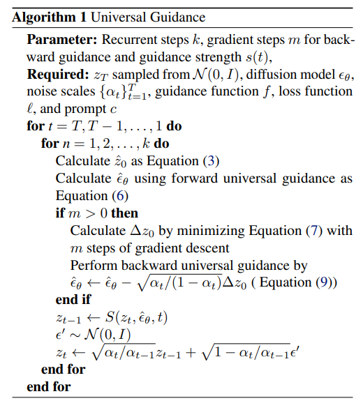
Universal guidance

(Bansal et al. 2023) extend classifier guidance from (Dhariwal, Nichol, 2021), with the idea that image sampling can be guided with any auxiliary network: the predicted noise to substract from the signal is “shifted” with the gradients of a loss function.

Note: to keep coherence with the paper, I move back to using $z_t$ over $x_t$, the noisy input from the diffusion forward process.

Forward universal guidance: given a guidance function $f$ and a loss $\ell$, the predicted noise is updated as:

\[\begin{equation} \tag{5} \hat{\epsilon}_{\theta}(z_{t},t)=\epsilon_{\theta}(z_{t},t)+\sqrt{1-\alpha_{t}}\nabla_{z_{t}}\ell_{c e}(c,f_{c l}(z_{t})) \end{equation}\] \[\begin{equation} \tag{6} \hat{\epsilon}_{\theta}(z_{t},t)=\epsilon_{\theta}(z_{t},t)+s(t)\cdot\nabla_{z_{t}}\ell(c,f(\hat{z}_{0})) \end{equation}\] \[\begin{align*} \nabla_{z_{t}}\ell(c,f(\hat{z_{0}}))=\nabla_{z_{t}}\ell\left(z,f\left(\frac{z_{t}-\sqrt{1-\alpha_{t}}\epsilon_{\theta}(z_{t},t)}{\sqrt{\alpha_{t}}}\right)\right) \end{align*}\]

Where $c$ is e.g. a classifier label as in (Dhariwal, Nichol, 2021). From equation $(6)$, $f$ is applied to the clean, denoised data point $\hat{z_0}$ instead of $z_t$ from equation $(5)$, as the auxiliary network may not work well on noisy data. $s(t)$ is a coefficient controlling the “guidance strength”: increasing this parameter, however, can excessively shift the generated samples out of the data manifold.

Backward universal guidance: in equation $(6)$ we compute $\hat{z_0} + \Delta z_0$, which directly minimizes $\ell$, instead of $\nabla_{z_{t}}\ell(c,f(\hat{z}_{0}))$. The guided denoising prediction results as:

\[\begin{equation}\tag{9} \tilde{\epsilon} = \epsilon_{\theta}\big(\mathcal{z}_{t},t\big) - \sqrt{\alpha_{t}/\big(1\,-\, \alpha_{t}\big)}\Delta\mathcal{z}_{0} \end{equation}\]

So $\Delta z_0$ is direction that best minimizes $\ell$ and it can achieved with m-step gradient-descent starting from $\Delta = 0$:

\[\begin{equation} \tag{7} \Delta z_0 = arg min_{\Delta} \ell(c,f(\hat{z}_{0} + \Delta) \end{equation}\]

Eventually:

\[\begin{equation} \tag{8} \mathcal{z}_{t} = \sqrt{\alpha_{t}}\big(\hat{z}_{0}\,+\,\Delta\mathcal{z}_{0}\big)\,+\,\sqrt{1\,-\,\alpha_{t}}\tilde{\epsilon} \end{equation}\]

With respect to forward universal guidance, gradient descent in $(7)$ results also cheaper than computing $(6)$.

A major issue is the lack of “realness” in generated samples when the guidance function causes excessive information loss: synthetic images can exhibit artifacts and strange distortions.

Consequently, at each sampling step, gaussian noise $\epsilon^{\prime}\sim\mathcal{N}(0,\mathrm{I})$ is iteratively added back to the computed $z_{t-1} = S(z_t, \hat{\epsilon_{\theta}}, t)$, such that:

\[\begin{equation} \tag{10} z_{t}^{\prime}=\sqrt{\alpha_{t}/\alpha_{t-1}}\cdot\ z_{t-1}+\sqrt{1-\alpha_{t}/\alpha_{t-1}}\cdot\epsilon^{\prime} \end{equation}\]

Each sampling step is repeated multiple teams to explore the data manifold and seek for better reconstructions.

The complete algorithm:

Source: (Bansal et al., 2023)

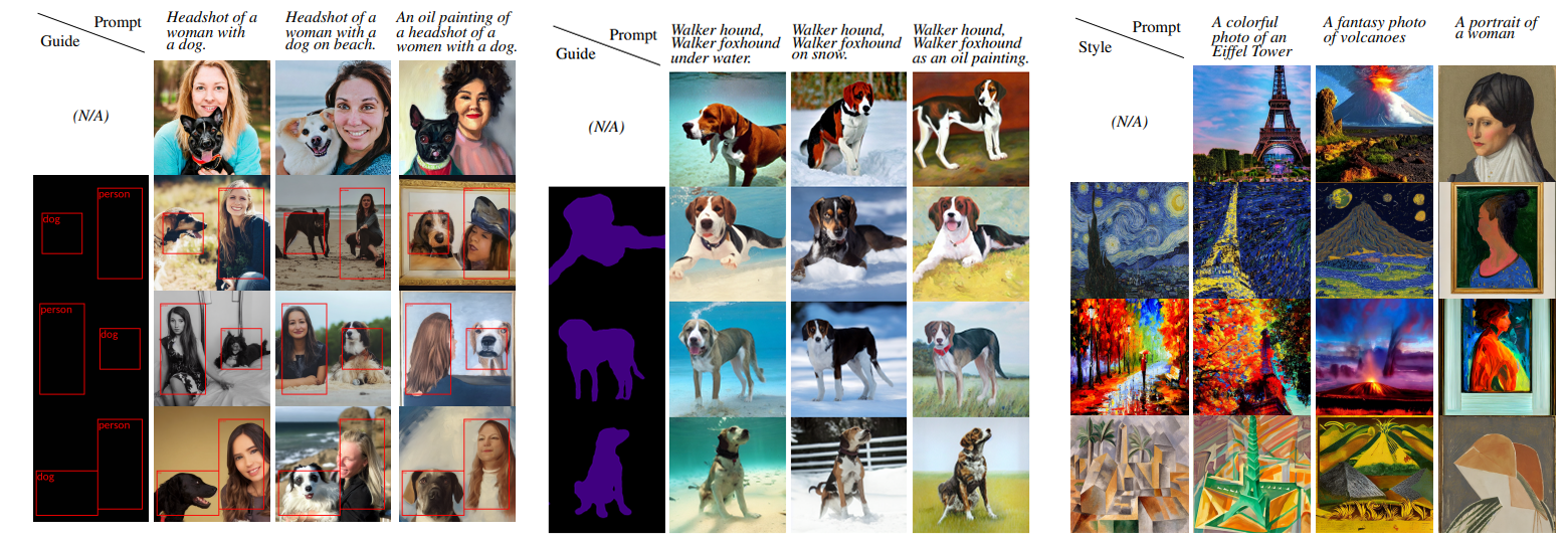
Experiments in the paper show the possibility to condition Stable Diffusion with networks for object detection, style transfer and image segmentation:

Source: (Bansal et al., 2023)

Conditioning with cross attention in Latent Diffusion

As already mentioned above, (Rombach et al., 2021) introduces a form of conditioning expanded to any modality encoded by a backbone network $\tau_{\phi}$ . The denoising network $\epsilon_{\theta}$ has a U-Net structure, cross attention is applied in each step $z_t \rightarrow z_{t-1}$ with the conditioning embedding from $\tau_{\phi}$.

Source: (Rombach et al., 2021)

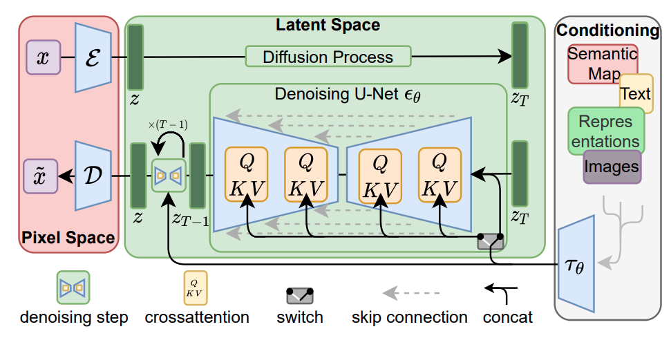
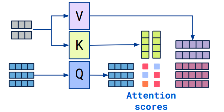
In cross attention, $z_t$ (grey) (assuming it’s embedded into a matrix with vector components) is mapped (with $W_i$ learnable) into a matrix of column keys $K = W_k \cdot z_t$ and a matrix of column values $V = W_v \cdot z_t$ ; the conditioning tokens of $\tau_\theta(c)$ are mapped into a matrix of column queries $Q = W_q \cdot \tau_\theta(c)$. Eventually, cross attention consists in $z_t$ “re-combined” according to its affinity with $\tau_\theta(c)$, more precisely: the value components of $z_t$ are linearly combined with the cross-attention scores given by $Q \cdot K^T$, thus:

\[V \cdot softmax(\frac{Q K^T}{\sqrt{d_k}})\]

With $d_k$ a normalizing constant.

Source: Jeagle et al. 2021